

Excel can do some crazy-cool things and make your life a whole lot easier once you learn how to use it.
That being said, in this article I’ll be teaching you one of the most basic, and most helpful, features of Microsoft Excel: formulas.
All Excel formulas must begin with an equal sign (=) followed by the operation that will be used to return the value. If you don’t start the formula with the equal sign, Excel will assume that you’re entering text, and not a formula.
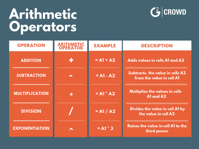
Formulas are written using arithmetic operators (addition, subtraction, multiplication, etc.) so that the values in the cell are combined to produce a single value as a result.
Now that you know about the arithmetic operators within a formula, let’s go over an example of entering an Excel formula.
In this example below, we are looking to calculate the charge for the first customer book order. Here are the steps I took to do so:

Reminder: Don’t forget that ALL formulas must start with the equal sign for Excel to recognize it as a formula.

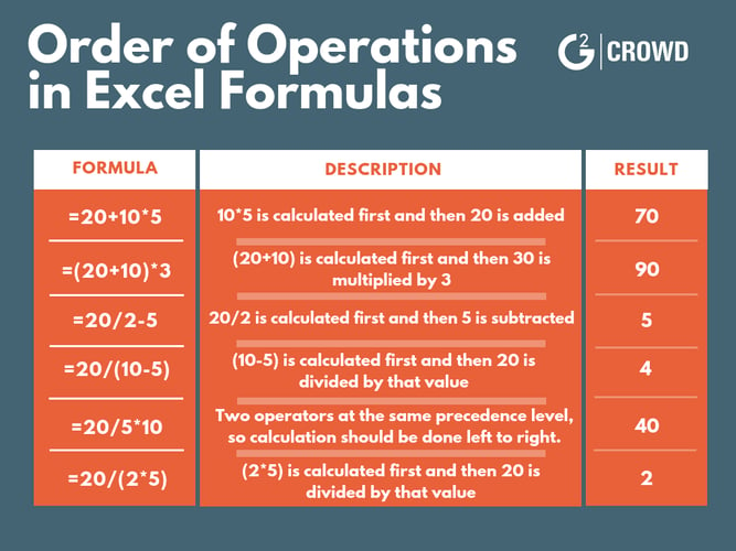
Sometimes your formulas will contain more than one arithmetic operator. In this case, you’ll need to consider the order of operations – the same ol’ order of operations you’ve learned in all of your math classes.
That being said, keep in mind that Excel will first calculate the value of any operation within parenthesis, followed by exponentiation (^), multiplication (*), and division (/), and finally addition (+) and subtraction (-).
Tip: Remember the acronym PEMDAS! Parenthesis, Exponentiation, Multiplication, Division, Addition, Subtraction.
| Tip: Interested in more Excel tips? Learn how to divide in Excel |
Let’s face it, we all make mistakes. And sometimes, you might need to go back and edit a formula after initially entering it. Don’t worry, it’s fairly easy!
In this example, I’m going to be editing my original formula from addition to multiplication.
Notice that when I highlight cell A3 my formula populates in the formula bar.

To edit this formula, click in the formula bar and edit the operator, changing it from addition to multiplication.

Now that you’ve edited what you needed to change, press ‘Enter’!

At some point there mere be a case where you’ll need to repeat the same formula throughout your worksheet. Good news – you won’t need to retype the formula over and over, you can copy and paste the formula from one cell to another!
Once you’ve copied a formula, it will be copied to the Excel Clipboard. Then once that formula is pasted, it will be moved from the Clipboard to the selected cell or cell range.
Excel will adjust the cell references in the formula to reflect the formula’s new location. This is because you want to copy the actions of the formula, not the specific value that the formula has generated in the first cell.
Below you’ll find an example of how to copy and paste your Excel formula. By doing this, you’ll save yourself time and avoid potential mistakes that may happen if you had retyped the formula separately.
In this example, we are looking to copy the original formula and paste it into the selected cells. Here are the steps I took to do so:

While I won’t cover Excel functions in-depth in this article, I will show you where to find the functions to simplify your Excel formulas and the most commonly used functions.
But before I jump into that, what is a function?
Excel’s functions are actually just preset formulas that are available to users.
While functions will auto-populate in a drop-down menu when you start to type your formula in the cell, you can also find the functions categorized at the top of your Excel page (see below).
You can search by clicking 'Insert Function' or browse the lists by clicking on each category separately.

There are dozens of useful functions available on Excel – here are the top 10 Excel functions you should start using today:
The SUM function (=SUM) is one of Excel's math and trig functions, and is used to add individual values, cell references, or ranges of cells.
The COUNT function is used to calculate the total amount of entries in a defined range that have numbers within the cell.
The AVERAGE function (=AVERAGE) is used to calculate the average of a selected cell range.
The IF function (=IF) is used to make logical comparisons between values and what you expect.
The SUMIF (=SUMIF) function is used to calculate the sum of values in a range that meet specified criteria.
SUMIF is for adding values that meet a specific criteria. For example, let’s say you want to find the sum of all values greater than 5 in your worksheet. This is a situation when you would use SUMIF.
The SUMIF function requires you to specify a range, a criteria, and a sometimes a sum range. The equation looks like this:
=SUMIF:(range,criteria,[sum_range])
The criteria is the condition that needs to be met. This can be a number, text, or an expression. For example, “Thursday”, “<10,” and “oranges” are all acceptable inputs. This is also a required input.
The sum range is the range of values, or cells, that will be added together if the range values meet the specified criteria. If this input is omitted, Excel will pull the sum of the range argument instead.
The Excel COUNTIF function (=COUNTIF) is one of Excel's statistical functions, and is used to count the number of cells that meet specified criteria.
There are many different scenarios where you may want to use Excel COUNTIF. I'll list a few below to help you start thinking strategically about how to incorporate this function into your work.
The COUNTIF function requires you to specify a range and a criteria. The equation looks like this:
=COUNTIF:(range,criteria)
The range is the cells you wish to analyze. For example, cells B12 through B150 would be a range.
The criteria is what you want to count. For example, any cell that contains the value 100.
You would write the function like this:
=COUNTIF:(B12:B150,100)
The AVERAGEIF function (=AVERAGEIF) is used to calculate the average of cells in a range that meet specified criteria.
The VLOOKUP function (=VLOOKUP) is used to find values in a table or range by row.
The CONCATENATE function (=CONCATENATE) is one of Excel's text functions, and is used to combine two or more strings of text into one string. This function will work for up to 30 strings of text at once.
The CONCATENATE function requires you to specify the cells you want to combine. The equation would look like this:
=CONCATENATE:(text1,text2)
Each "text" you specify will be from a different cell, for example:
=CONCATENATE:(A2,B2)
Press ENTER to complete the function. The days of manually combing through data to get a perfect spreadsheet are long gone!
The MAX function (=MAX) is used to return the largest value in a set of values. The MIN function (=MIN) is used to return the smallest value in a set of values.
Excel formulas can make your life a whole lot easier. They can save you time and most of all, a headache from having to do all of the math on your own.
When it comes to writing those formulas, keep these few tips in mind:
If possible, use functions in place of those long, complex formulas. Simplifying formulas with functions helps avoid mistakes when entering a formula, ensuring that the formula is making an accurate calculation.
For example, if you’re adding more than two or three cells together, you may consider using the SUM function to make sure you don’t improperly enter a cell and end up with an incorrect value.
Before entering the actual values, test your formula with simple values that you can calculate in your head to confirm that your formula is working as expected.
For example, say you're just learning how to subtract in Excel. Use 1’s or 10’s as your input values first – something easy to calculate in your head – to verify your formula was input correctly and is working as intended.
The cells will display the result of the formula, not the actual formula.
For example, say you’re looking to calculate a 7 percent interest rate on a value in B5. You could enter the formula =0.07*B5. However, this won’t show how the value is calculated. Instead, place the value 0.07 in a cell accompanied by a label and use the cell reference in the formula. So if you place 0.07 in cell B6, the formula =B6*B5 will calculate the interest value.
This allows others to easily see the interest rate as well as the resulting interest, ensuring that your formula is easy to understand and clearly solving the problem.
In this article we’ve covered what Excel formulas are and how to enter, edit, copy and paste, and simplify your Excel formulas – everything you need to know about using Excel formulas!
Excel isn't the only spreadsheet in the town. Explore the other top-rated spreadsheet software that is as easy as Excel.


Here's a situation I'm willing to bet you've been in.
 by Krithika Sathyamoorthy

The hardest part of a business letter isn’t knowing what it is; it’s writing one that feels...
.png) by Shreya Mattoo
by Shreya Mattoo

There are two types of people in this world: those who see a blank spreadsheet and panic, and...
 by Washija Kazim